Rectified Flow: Straight is Fast

Rectified flow learns ODEs as generative models by causalizing (or rectifying) an interpolation process that smoothly connects noise and data. This process naturally favors dynamics with straighter trajectories and hence fast Euler discretization, and can be repeated to further improve straightness.

Overview

This blog provides a brief introduction to rectified flow, based on Chapter 1 of these lecture notes. For more introduction, please refer to the original papers and these blogs.

Problem: Learning Flow Generative Models

Generative modeling can be formulated as finding a computational procedure that transforms a noise distribution, denoted by $\pi_0$, into an unknown data distribution $\pi_1$ observed from data. In flow models, this procedure is represented by an ordinary differential equation (ODE):

\[\dot{Z}_t = v_t(Z_t), \quad \forall t \in [0,1], \quad \text{starting from } Z_0 \sim \pi_0, \tag{1}\]

where $\dot{Z}_t = \mathrm dZ_t / \mathrm dt$ denotes the time derivative, and the velocity field $v_t(x) = v(x, t)$ is a learnable function to be estimated to ensure that $Z_1$ follows the target distribution $\pi_1$ when starting from $Z_0 \sim \pi_0$. In this case, we say that the stochastic process $Z = \{Z_t\}$ provides an (ODE) transport from $\pi_0$ to $\pi_1$.

It is important to note that, in all but trivial cases, there exist infinitely many ODE transports from $\pi_0$ to $\pi_1$, provided that at least one such process exists. Thus, it is essential to be clear about which types of ODEs we should prefer.

One option is to favor ODEs that are easy to solve at inference time. In practice, the ODEs are approximated using numerical methods, which typically construct piecewise linear approximations of the ODE trajectories. For instance, a common choice is the Euler method:

\[\hat{Z}_{t+\epsilon} = \hat{Z}_t + \epsilon v_t(\hat{Z}_t), \quad \forall t \in \{0, \epsilon, 2\epsilon, \dots, 1\}, \tag{2}\]

where $\epsilon > 0$ is a step size. Varying the step size $\epsilon$ introduces a trade-off between accuracy and computational cost: smaller $\epsilon$ yields higher accuracy but requires more computation steps. Therefore, we should seek ODEs that can be approximated accurately even with large step sizes.

Figure 1. Lady Windermere's fan for illustration of error accumulation in Euler method trajectories, starting from various initial points and deviating from the true solution curve over time.

The ideal scenario arises when the ODE follows straight-line trajectories, in which case Euler approximation yields zero discretization error regardless of the choice of step sizes. In such cases, the ODE, up to time reparameterization, should satisfy:

\[Z_t = t Z_1 + (1 - t) Z_0, \quad \implies \quad \dot{Z}_t = Z_1 - Z_0.\]

These ODEs, known as straight transports, enable fast generative models that can be simulated in a single step. We refer to the resulting pair $(Z_0, Z_1)$ as a straight coupling of $\pi_0$ and $\pi_1$. In practice, we may not achieve perfect straightness, but we can aim to make the ODE trajectories as straight as possible to maximize computational efficiency.

Rectified Flow

To construct a flow transporting $\pi_0$ to $\pi_1$, let us assume that we are given an arbitrary coupling $(X_0, X_1)$ of $\pi_0$ and $\pi_1$, from which we can obtain empirical draws. This can simply be the independent coupling with law $\pi_0 \times \pi_1$, as is common in practice when we have access to independent samples from $\pi_0$ and $\pi_1$. The idea is to take $(X_0, X_1)$ and convert it to a better coupling generated by an ODE model. Optionally, we can then iteratively repeat this process to further enhance desired properties, such as straightness.

Rectified flow is constructed in the following ways:

Build Interpolation:

The first step is to build an interpolation process $\{X_t\} = \{X_t : t \in [0, 1]\}$ that smoothly interpolates between $X_0$ and $X_1$. Although general choices are possible, let us consider the canonical choice of straight-line interpolation:

\[X_t = t X_1 + (1 - t) X_0.X_t = t X_1 + (1 - t) X_0.\]

Here the interpolation $\{X_t\}$ is a stochastic process generated in an “anchor-and-bridge” way: we first sample the endpoints $X_0$ and $X_1$ and then sample the intermediate trajectory connecting them.

Marginal Matching:

By construction, the marginal distributions of $X_0$ and $X_1$ match the target distributions $\pi_0$ and $\pi_1$ through the interpolation process $\{X_t\}$. However, $\{X_t\}$ is not a causal ODE process like $\dot{Z}_t = v_t(Z_t)$, which generate the output $Z_1$ by evolving forward in time from $Z_0$. Instead, generating $X_t$ requires knowledge of both $X_0$ and $X_1$, rather than evolving solely from $X_0$ as $t$ increases.

This issue can be resolved if we can convert $\{X_t\}$ somehow into a causal ODE process while preserving the marginal distributions of $X_t$ at each time $t$. Note that since we only care about the output $X_1$, we only need to match the marginal distributions of $X_t$ at each individual time $t$. There is no need to match the trajectory-wise joint distribution of $\{X_t\}$.

Perhaps surprisingly, marginal matching can be achieved by simply training the velocity field $v_t$ of the ODE model $\dot{Z}_t = v_t(Z_t)$ to match the slope $\dot{X}_t$ of the interpolation process via:

\[\min_v \int_0^1 \mathbb{E} \left[ \left\| \dot{X}_t - v_t(X_t) \right\|^2 \right] \mathrm dt. \tag{3}\]

The theoretical minimum is achieved by:

\[v_t^*(x) = \mathbb{E} \left[ \dot{X}_t \mid X_t = x \right],\]

which is the conditional expectation of the slope $\dot{X}_t$ for all the interpolation trajectories passing through a given point $X_t = x$. If multiple trajectories pass point $X_t=x$, the velocity $v_t^*(x)$ is the average of $\dot X_t$ for these trajectories.

With the canonical straight interpolation $X_t = t X_1+(1-t)X_0$, we have $\dot{X}_t = X_1 - X_0$ by taking the derivative of $X_t$ with respect to $t$. It yields:

\[\min_v \int_0^1 \mathbb{E} \left[ \| \dot{X}_t - v_t(X_t) \|^2 \right] \mathrm dt, \quad X_t = t X_1 + (1 - t) X_0.\]

In practice, the optimization in (3) can be efficiently solved even for large AI models when $v$ is parameterized as modern deep neural nets. This is achieved by leveraging off-the-shelf optimizers with stochastic gradients, computed by drawing pairs $(X_0, X_1)$ from data, sampling $t$ uniformly in $[0, 1]$, and then computing the corresponding $(X_t, \dot{X}_t)$ using the interpolation formula.

Notation. A stochastic process $X_t = X(t, \omega)$ is a measurable function of time $t$ and a random seed $\omega$ (with, say, distribution $\mathbb{P}$). In the case above, the end points are the random seed, i.e., $\omega = (X_0, X_1)$. The slope is given by $\dot{X}_t = \partial_t X(t, \omega)$ as the partial derivative of $X$ w.r.t. $t$, which is also a function of the same random seed. The expectation in the loss, written in full, is
\[\mathbb{E}_{\omega \sim \mathbb{P}} \left[ \left\| \partial_t X(t, \omega) - v_t(X(t, \omega)) \right\|^2 \right].\]
In writing, we often omit the random seed. Whenever we take the expectation, it averages out all random sources inside the brackets except for those explicitly included in the conditioning.

Figure 2. Rectified flow between $\pi_0$ and $\pi_1$. Blue and pink lines represent trajectories, colored by the mode they are associated with for visualization.

We illustrate the intuition in Fig.2:

In the interpolation process $\{X_t\}$, different trajectories may have intersecting points, resulting in multiple possible values of $\dot X_t$ associated with a same point $X_t$ due to uncertainty about which trajectory it was drawn from (Fig.2a).
In contrast, by the definition of an ODE $\dot{Z}_t = v_t^*(Z_t)$, the update direction $\dot{Z}_t$ at each point $Z_t$ is uniquely determined by $Z_t$, making it impossible for different trajectories of ${Z_t}$ to intersect and then diverge along different directions.
Hence at these intersection points of $\{X_t\}$ where ${\dot X_t}$ is uncertain and non-unique, the ODE $\{Z_t\}$ “derandomizes” the update direction by following the conditional expectation $\displaystyle v_t^*(X_t) = \mathbb{E}[\dot{X}_t \mid X_t].$ Consequently, the trajectories of the ODE “reassemble” the interpolation trajectories in a way that avoids intersections. See Fig.2(b).
Since ODE trajectories ${Z_t}$ cannot intersect, they must curve at potential intersection points to “rewire” the original interpolation paths and avoid crossing.

Rectified Flow. For any time-differential stochastic process $\{X_t\} = \{X_t : t \in [0, 1]\}$, we call the ODE process:
\[\dot{Z}_t = v_t^*(Z_t) \quad \text{with} \quad v_t^*(x) = \mathbb{E} \left[ \dot{X}_t \mid X_t = x \right], \quad Z_0 = X_0\]
the rectified flow induced by $\{X_t\}$. We denote it as:
\[\{Z_t\} = \texttt{Rectify}(\{X_t\}).\]

Figure 3 illustrates a close-up view of how rectification “rewires” interpolation trajectories. Consider two “beams” of interpolation trajectories intersecting to form the “region of confusion” (shaded area in the middle). Within this region, a particle moving along the rectified flow follows the averaged direction $v^*_t$. Upon exiting, the particle joins one of the original interpolation streams based on its exit side and continues moving. Since rectified flow trajectories do not intersect within the region, they remain separated and exit from their respective sides, effectively “rewiring” the original interpolation trajectories.

What makes rectified flow $\{Z_t\}$ useful is that it preserves the marginal distributions of $\{X_t\}$ at each point while resulting in a “better” coupling $(Z_0, Z_1)$ in terms of optimal transport:

Marginal Preservation

The $\{X_t\}$ and its rectified flow $\{Z_t\}$ share the same marginal distributions at each time $t \in [0, 1]$, that is:
\[\text{Law}(Z_t) = \text{Law}(X_t), \quad \forall t \in [0, 1],\]
where $\text{Law}(X_t)$ denotes the probability distribution (or law) of random variable $X_t$.

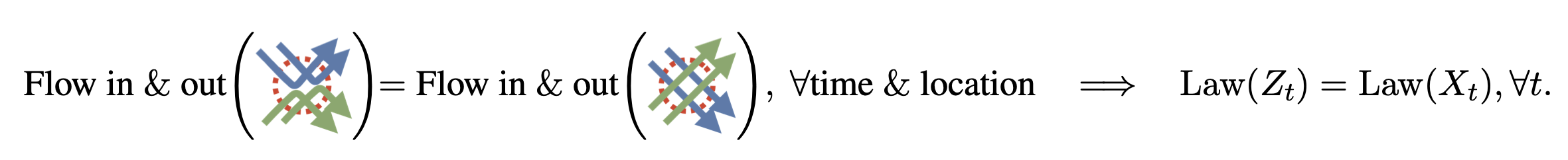
Intuitively, by the definition of $v_t$ in (1), the total amount of mass flow entering and exiting every infinitesimal volume in the space is equal under the dynamics of $X_t$ and $Z_t$. This ensures that the two processes yield the same marginal distributions, even though the flow directions may differ.
Transport Cost

The start-end pairs $(Z_0, Z_1)$ from the rectified flow $\{Z_t\}$ guarantee to yield no larger transport cost than $(X_0, X_1)$, simultaneously for all convex cost functions $c$:
\[\mathbb{E} \left[ c(Z_1 - Z_0) \right] \leq \mathbb{E} \left[ c(X_1 - X_0) \right], \quad \forall \text{convex } c : \mathbb{R}^d \to \mathbb{R}.\]
Intuitively, it is because disentangling the intersections reduces the length of the trajectories by triangle inequality:

Reflow

While rectified flows tend to favor straight trajectories, they are not perfectly straight. As in Fig.2 (a), the flow makes turns at intersection points of the interpolation trajectories $\{X_t\}$. How can we further improve the flow to achieve straighter trajectories and hence speed up inference?

A key insight is that the start-end pairs $(Z_0, Z_1)$ generated by rectified flow, called the rectified coupling of $(X_0, X_1)$, form a better and “straighter” coupling compared to $(X_0, X_1)$. This is because if we connect $Z_0$ and $Z_1$ with a new straight-line interpolation, it would yield fewer intersection points. Hence, training a new rectified flow based on this interpolation would result in straighter trajectories, leading to faster inference.

Formally, we apply the $\texttt{Rectify}(·)$ procedure recursively, yielding a sequence of rectified flows starting from $(Z_0^0, X_1^0) = (X_0, X_1)$:

\[\texttt{Reflow:} \quad \quad \{Z_t^{k+1}\} = \texttt{Rectify}(\texttt{Interp}(Z_0^k, Z_1^k)),\]

where $\text{Interp}(Z_0^k, Z_1^k)$ denotes an interpolation process given $(Z_0^k, Z_1^k)$ as the endpoints. We call $\{Z_t^k\}$ the $k$-th rectified flow, or simply the $k$-rectified flow, induced from $(X_0, X_1)$.

This reflow procedure is proved to “straighten” the paths of rectified flows in the following sense: Define the following measure of straightness of $\{Z_t\}$:

\[S(\{Z_t\}) = \int_0^1 \mathbb{E} \left[ \|Z_1 - Z_0 - \dot{Z}_t\|^2 \right] \mathrm dt,\]

where $S(\{Z_t\})$ is a measure of the straightness of $\{Z_t\}$, with $S(\{Z_t\}) = 0$ corresponding to straight paths. Then it can be found in paper that

\[\mathbb{E}_{k \sim \text{Unif}(\{1, \dots, K\})} \left[S(\{Z_t^k\})\right] = \mathcal{O}(1 / K),\]

which suggests that the average of $S(\{Z_t^k\})$ in the first $K$ steps decay with an $\mathcal{O}(1 / K)$ rate.

Note that reflow can begin from any coupling $(X_0, X_1)$, so it provides a general procedure for straightening and thus speeding up any given dynamics while preserving the marginals.

As shown in Fig.2 (c), after applying the “Reflow” operation, the trajectories become straighter than the original rectified flow $Z_t$.

Reflow and Shortcut Learning. Intuitively, reflow resembles shortcut learning in humans: once we solve a problem for the first time, we learn to go directly to the solution, enabling us to solve it more quickly the next time.