Flow to Diffusion: Langevin is a Guardrail

It is known that we can convert between diffusion (SDE) and flow (ODE) models at inference time without retraining. But how is this possible? What is the intuition and purpose? What are the pros and cons of diffusion vs. flow?

Overview

Rectified flow (RF) provides a deterministic ODE (a.k.a. flow) model, of the form \(\mathrm d Z_t = v_t(Z_t)\mathrm d t\), which generates the data \(Z_1\) starting from initial noise \(Z_0\). This approach simplifies the generative process compared to diffusion models, which rely on a stochastic differential equation (SDE) to generate data from noise, such as DDPM and score-based models.

Nonetheless, since the work of DDIM and probability-flow ODEs, the boundary between flow and diffusion models has been known as blurry. These prior works showed that an SDE can be converted into an ODE during inference without retraining the model. Conversely, starting from ODE models, it is also possible to revert the process and convert the RF ODE into SDEs to obtain stochastic samplers at inference time. This raises several questions:

Why and how is it possible to convert between SDEs and ODEs? What is the intuition?
Why would we bother to add diffusion noise given that ODEs are simpler and faster? What are the pros and cons of diffusion vs. flow?

This blog post explores these questions. For a more detailed discussion, see Chapter 5 of the Rectified Flow Lecture Notes. Related works include DDIM, score-based SDEs, EDM.

Stochastic Samplers = RF + Langevin

Given a coupling \((X_0, X_1)\) of noise and data points, rectified flow defines an interpolation process, such as \(X_t = t X_1 + (1 - t) X_0\), and “rectifies” or “causalizes” it to yield an ODE model \(\mathrm{d} Z_t = v_t(Z_t) \, \mathrm{d} t\) initialized from \(Z_0 = X_0.\) The velocity field is given by \(v_t(z) = \mathbb{E}[\dot{X}_t \mid X_t = z],\) which is estimated by minimizing a loss like \(\mathbb{E}_{t, X_0, X_1} [ \| \dot{X}_t - v_t(X_t) \|^2 ].\)

A key property of the RF ODE is its marginal preserving property: the distribution of \(Z_t\) on the ODE trajectory matches the distribution of \(X_t\) on the interpolation path at each time \(t\). This is ensured by constructing the velocity field \(v_t\) in an inductive way: if the distributions of \(X_t\) and \(Z_t\) match up to a given time, the constructed \(v_t\) guarantees they will continue to match at the next infinitesimal step. As a result, the final output \(Z_1\) of the ODE follows the same distribution as \(X_1\), the target data distribution. By being “scheduled to do the right thing at the right time,” the process guarantees the correct final result.

However, one challenge is that errors can accumulate over time as we solve the ODE \(\mathrm{d} Z_t = v_t(Z_t) \mathrm{d} t\) in practice. These errors arise from both model approximations and numerical discretization, causing drift between the estimated distribution and the true distribution. The problem can compound: if the estimated trajectory \(\hat{Z}_t\) deviates significantly from the distribution of \(X_t\), the update direction \(v_t(\hat{Z}_t)\) becomes less accurate and can further reinforce the deviation.

To address this problem, we may introduce a feedback mechanism to correct the errors. One such approach is to use Langevin dynamics.

Langevin Dynamics. For a density function \(\rho^*(x)\), its (discrete-time) Langevin dyamics is
\[\hat{Z}_{t+\epsilon} = \hat{Z}_t + \epsilon \sigma_t^2 \nabla \log \rho^*(\hat{Z}_t) + \sqrt{2\epsilon}\,\sigma_t\,\xi_t,\quad \xi_t \sim \mathtt{Normal}(0, I),\]
where \(\sigma_t\) is the diffusion coefficient, and \(\epsilon>0\) is the step size. Intuitively, this update is gradient ascent on log probability \(\log \rho^*\) with Gaussian noise perturbations of variance \(\epsilon\) at each step. Langevin dynamics provides an approximate method to draw samples from \(\rho^*\) because, under regularity conditions, the distribution of \(Z_t\) converges to \(\rho^*\) as \(t \to +\infty\) and \(\epsilon \to 0\).

When the step size \(\epsilon\) approaches to zero, the continuous-time limit of this update is written as a stochastic differential equation (SDE):
\[\mathrm{d} Z_t = \sigma_t^2 \nabla \log \rho^*(Z_t) \mathrm{d} t + \sqrt{2}\sigma_t \mathrm{d} W_t,\]
where \(\{W_t\}\) is a Brownian motion, which has independent increments (for every \(t > 0\), the future increments \(\{W_{t+u} - W_t,\, u \ge 0\}\) are independent of the past trajectory \(\{W_s,\, s < t\}\)) and Gaussian increments \(\bigl(W_{t+u} - W_t \sim \mathcal{N}(0, u)\bigr)\).

We do not need to delve deeply into SDE theory here. It suffices to substitute the SDE with the discrete-time update, understanding that the SDE represents the continuous-time limit of the discrete-time update in a suitable sense, which mathematicians have already clarified.

Let \(\rho_t\) be the density function of \(X_t\), representing the true distribution that we aim to follow at time \(t\). At each time step \(t\), we can in principle apply a short segment of Langevin dynamics to adjust the trajectory’s distribution toward \(\rho_t\):

\[\mathrm{d} Z_{t, \tau} = \sigma_t^2 \nabla \log \rho_t(Z_{t, \tau}) \, \mathrm{d} \tau + \sqrt{2} \, \sigma_t \, \mathrm{d} W_\tau, \quad \tau \geq 0,\]

where \(\tau\) is an auxiliary time scale for the Langevin dynamics. This yields a double-loop algorithm in which the system is simulated to equilibrium \((\tau \to \infty)\) at each \(t\) before moving on to the next time point.

In rectified flow, however, the trajectory is already close to \(\rho_t\) at each time step \(t\). Therefore, a single step of Langevin dynamics can be sufficient to mitigate the drift. This allows us to directly integrate Langevin corrections into the rectified flow updates, yielding a combined SDE:

\[\mathrm{d}{Z}_t = \underbrace{v_t({Z}_t) \,\mathrm{d} t}_{\textcolor{blue}{\text{Rectified Flow}}} + \underbrace{\sigma_t^2 \nabla \log \rho_t({Z}_t)\,\mathrm{d} t + \sqrt{2}\,\sigma_t\,\mathrm{d}W_t}_{\textcolor{red}{\text{Langevin Dynamics}}} ,\quad \tilde{Z}_0 = Z_0.\]

This combined SDE achieves two primary objectives:

The rectified flow drives the generative process forward as intended.
The Langevin component acts as a negative feedback loop, correcting distributional drift without bias when \(\tilde{Z}_t\) and \(\rho_t\) are well aligned.

When the simulation is accurate, Langevin dynamics naturally remain in equilibrium, avoiding unnecessary changes to the distribution. However, if deviations occur, this mechanism guides the estimate back on track, enhancing the robustness of the inference.

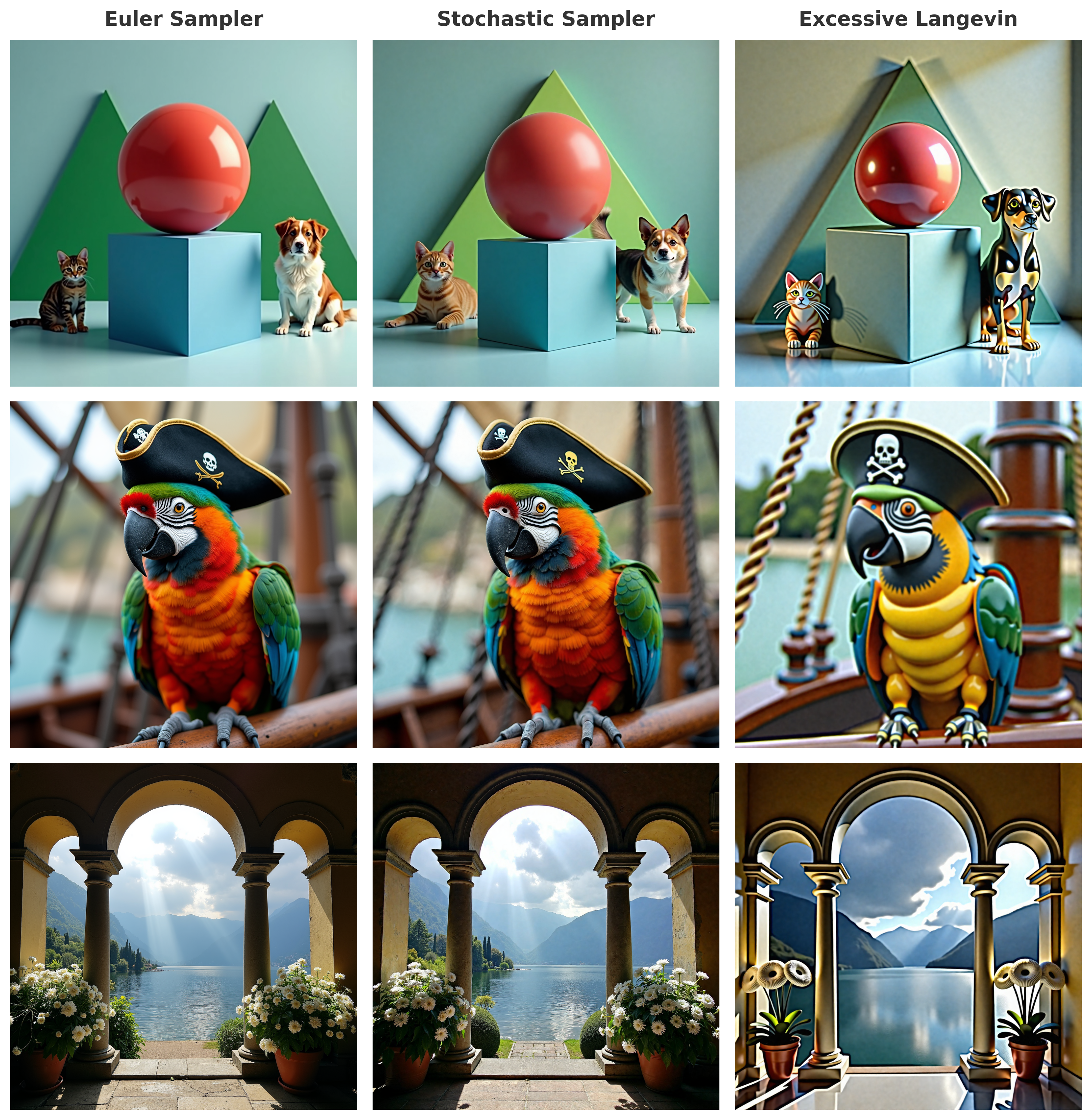
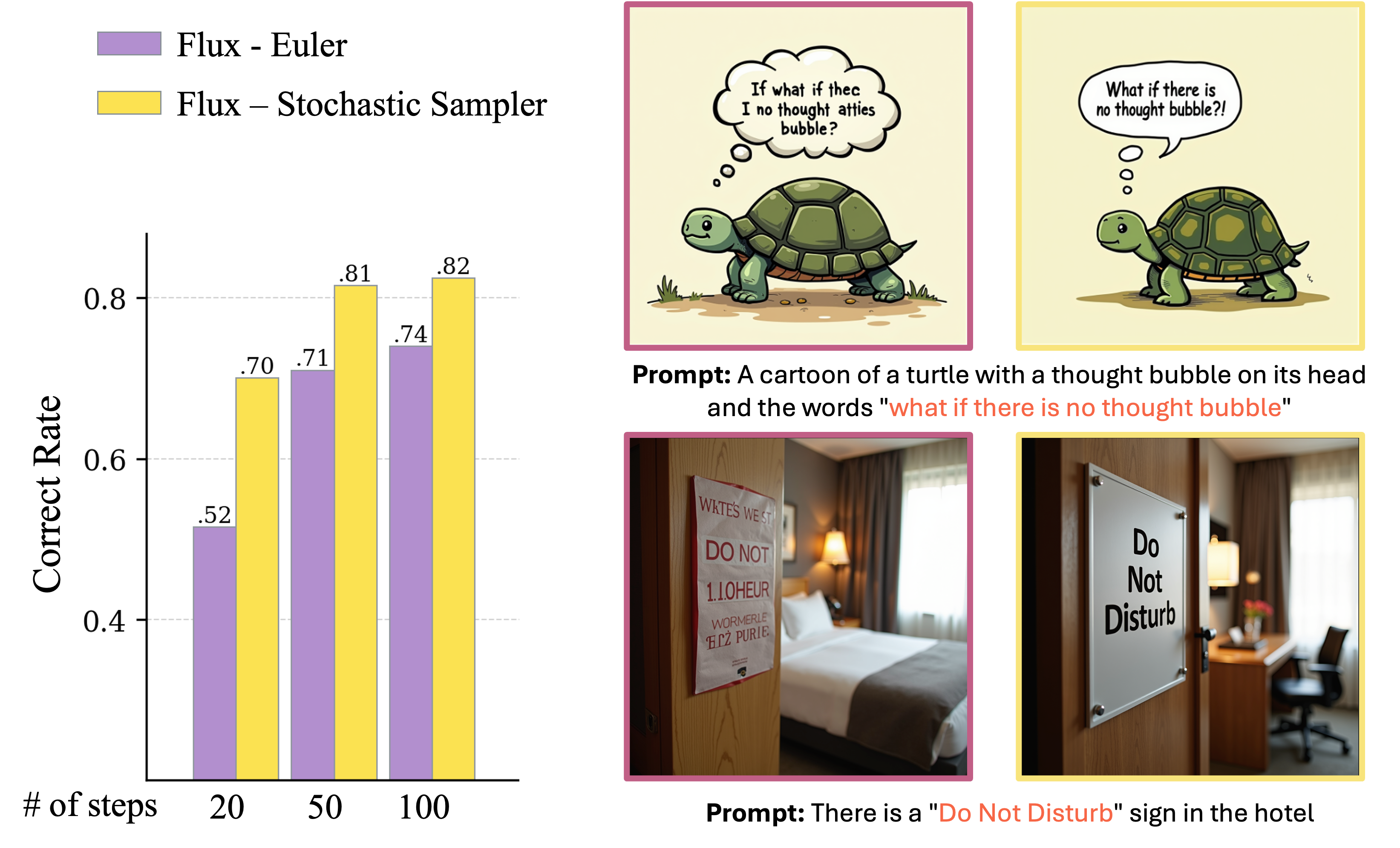
Figure 1. Illustration of the (normalized) score function \(\nabla \log \rho_t\) along the SDE trajectories. We can see that \(\nabla \log \rho_t\) points toward high-density regions, helping guide trajectories back to areas of higher probability whenever deviations occur.

Figure 2. Comparing two sampling methods. On the left, we apply Euler discretization to the deterministic ODE using a "poor" \(v_t\) (due to early stopping), resulting in many outliers. On the right, the Euler–Maruyama method simulates the SDE, effectively suppressing outliers through the feedback of the score function.

This correction mechanism also has an effect on state-of-the-art text-to-image generation. In a recent work, we found that stochastic samplers improve text rendering quality over deterministic samplers in SOTA models such as Flux. Moreover, they produce images that better reflect the text prompt. The figure below shows that using a stochastic sampler on the Flux model consistently outperforms the deterministic Euler sampler in text rendering quality across all step sizes. The right side shows qualitative examples demonstrating the enhanced text rendering achieved by the stochastic sampler.

SDEs with Tweedie’s formula

Solving the SDEs requires estimating the score function \(\nabla \log \rho_t\) in addition to the RF velocity \(v_t\). However, in certain special cases, the score function can be estimated from \(v_t\), thus avoiding the need to retrain an additional model. This enables a training-free conversion between ODEs and SDEs.

Specifically, if the rectified flow is induced by an affine interpolation \(X_t = \alpha_t X_1 + \beta_t X_0\), where \(X_0\) and \(X_1\) are independent (i.e., \(X_0 \perp\!\!\!\perp X_1\)) and \(X_0\) follows a standard Gaussian distribution, then by Tweedie’s formula, we have

\[\nabla \log \rho_t(x) = -\frac{1}{\beta_t} \mathbb{E}[X_0 \mid X_t = x].\]

On the other hand, the RF velocity is given by

\[v_t(x) = \mathbb{E}[\dot{X}_t \mid X_t = x] = \mathbb{E}[\dot{\alpha}_t X_1 + \dot{\beta}_t X_0 \mid X_t = x].\]

Using this, we can express \(\mathbb{E}[X_0 \mid X_t = x]\) in terms of \(v_t(x)\) and obtain

\[\nabla \log \rho_t(x) = \frac{\alpha_t v_t(x) - \dot{\alpha}_tx}{\lambda_t\beta_t}, \quad \text{where } \lambda_t = \dot{\alpha}_t \beta_t - \alpha_t \dot{\beta}_t.\]

As a result, the SDE takes the form

\[\mathrm d Z_t = v_t(Z_t)\mathrm d t + \gamma (\alpha_t v_t (x) - \dot \alpha_t x) \mathrm{d} t + \sqrt{2 \lambda_t \beta_t \gamma_t} \mathrm{d} W_t,\]

where we set \(\sigma_t^2 = \lambda_t \beta_t \gamma_t\).

In the case of straight interpolation \(X_t = t X_1 + (1-t)X_0\), we have \(\nabla \log \rho_t(x) = \frac{t v_t(x) - x}{1-t}\), leading to

\[\mathrm d Z_t = v_t(Z_t)\mathrm d t + \gamma_t (t v_t (x) - x) \mathrm{d} t + \sqrt{2 \gamma_t (1-t) } \mathrm{d} W_t.\]

The SDE of DDPM and the score-based SDEs can be recovered by setting \(\gamma_t = 1 / \alpha_t\) and \(\alpha^2_t + \beta_t^2 = 1\), giving

\[\mathrm{d} Z_t = 2 v_t(Z_t) \, \mathrm{d} t - \frac{\dot{\alpha}_t}{\alpha_t} Z_t \, \mathrm{d} t + \sqrt{2 \frac{\dot \alpha_t}{\alpha_t}} \mathrm{d} W_t.\]

Diffusion May Cause Over-Concentration

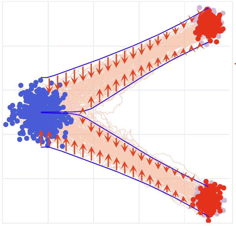
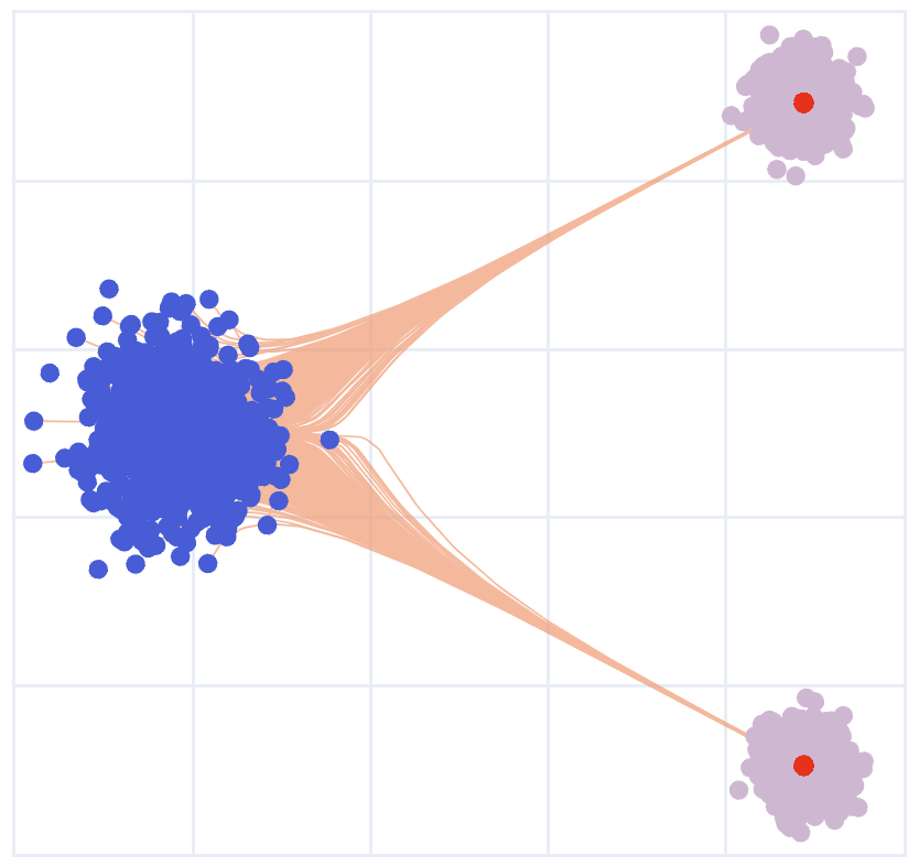
Although things work out nicely in theory, we need to be careful that the introduced score function \(\nabla \log \rho_t(x)\) itself has errors, and it may introduce undesirable effects if we rely on it too much (by using a large \(\sigma_t\)). This is indeed the case in practice. As shown in the figure below, when we increase the noise magnitude \(\sigma_t\), the generated samples tend to cluster closer to the centers of the Gaussian modes.

So, larger diffusion yields more concentrated results? This appears counterintuitive at first glance. Why does this happen?

To see this, assume the estimated velocity field is \(\hat v_t \approx v_t\). The corresponding estimated score function from Tweedie’s formula becomes

\[\nabla \log \hat \rho_t(x) = \frac{1}{\lambda_t \beta_t} \left( \alpha_t \hat v_t(x) - \dot{\alpha}_t x \right).\]

Because \(\beta_t\) must converge to 0 as \(t \to 1\), the estimated score function \(\nabla \log \hat{\rho}_t(x)\) would diverge to infinity in this limit. On the other hand, the true magnitude of \(\nabla \log \rho_t(x)\) may be finite, thus being significantly overestimated when \(t\) is close to 1. Since \(\nabla \log \rho_t(x)\) point toward the centers of mass of clusters, its overestimation leads to an overly concentrated distribution around these centers.

Role of Noise. In summary, the Langevin guardrail can become too excessive, causing over-concentration. It is the score function \(\nabla \log \rho_t(x)\) that drives this concentration, rather than the noise itself, as one might initially assume from the ODE vs. SDE dichotomy. The noise component in Langevin dynamics compensates for the concentration induced by the score function, but it does not necessarily prevent it when the score is overestimated.

In the context of text-to-image generation, this over-concentration effect often produces overly smoothed images, which sometimes appear cartoonish. Such over-smoothing eliminates fine details and high-frequency variations, resulting in outputs with a blurred appearance. The figure below illustrates these differences: samples generated using the Euler sampler exhibit more high-frequency details, as seen in the texture of the parrot’s feathers and the structure of the smoke.